Complementary Cumulative Distribution Function (CCDF) in Modern Modulation Measurements

As utilization of wireless communications has accelerated over the past few years, the push to make efficient use of the limited amount of spectrum available has led to the development of more complex modulation schemes. Waveforms have continued to evolve from constant-envelope GSM and IS-95 CDMA of yesteryear to higher order M-QAM and OFDM, which can now be found in all things 5G, Wi-Fi, Satcom and Bluetooth. Minimizing the RF power required is essential to reducing heat dissipation, extending battery life, lowering costs, increasing spectral efficiency and reducing overall system complexity.

Measuring RF power has been standard practice for many years. The most fundamental RF power measurements simply capture a single value at a given point in time. How RF power is measured depends on a priori knowledge of the signal being measured. For example, is it a CW or pulsed waveform? What are the losses in the system? What noise is present? What accuracy and repeatability are required? Perhaps most importantly, how often does the RF signal reach a given peak power, compared to its average power? Read on for a discussion of complex waveform characteristics and some of the functions that are utilized in measuring them.

All that Noise about OFDM

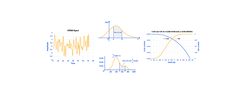
In the time domain, as illustrated by the OFDM waveform in Figure 1, modern RF signals look more like noise and less like the AM, FM, and pulse-modulated waveforms of old. It follows that there is a need to describe the RF power of these complex signals in a meaningful way. Instead of measuring RF power at a single point in time, their RF power can be characterized with statistics.

Figure 1: 16-QAM OFDM waveform comprised of 64 data points shown in the time domain

The Probability Density Function (PDF)

Statistics can be employed to show the distribution of RF power in three popular ways; the probability density function (PDF), the cumulative distribution function (CDF) and the complementary cumulative distribution function (CCDF). Each of these statistical measures expresses the peak-to-average power ratio (PAPR) of the RF signal. The longer the RF system is operated above its average power or the longer it spends near its peak value, the more stress is placed on the components.

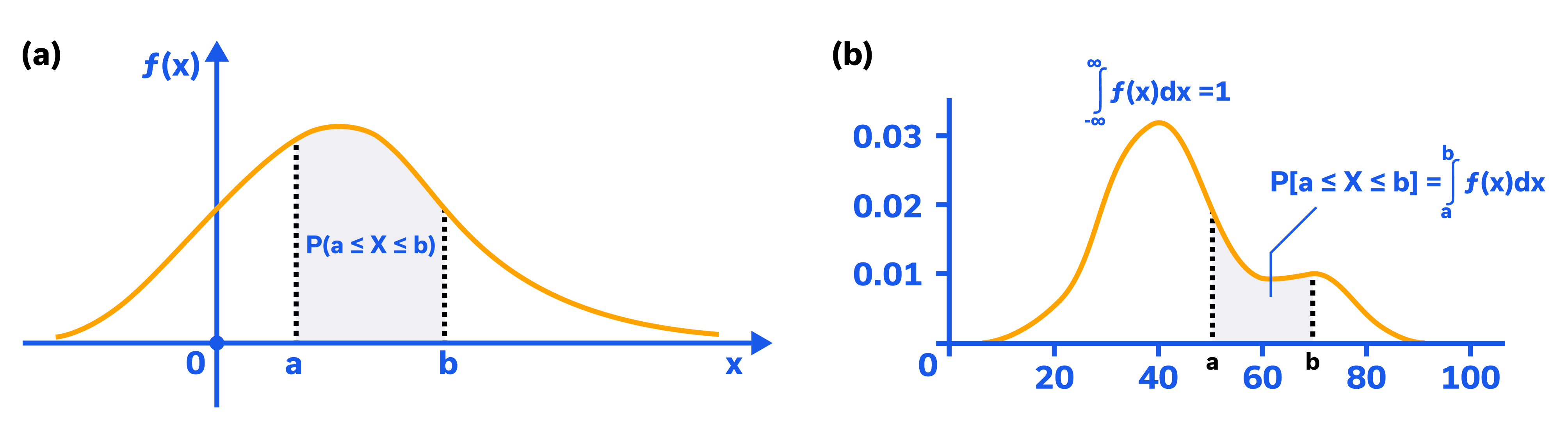
For the following explanation, refer to the skewed distribution curve in Figure 2(a) and the bimodal distribution curve in Figure 2(b). Figure 2(a) identifies the probability that X lies between a and b inclusive, P(a ≤ X ≤ b). Figure 2(b) shows that the probability density function is determined by integrating the statistical distribution curve f(x) between the two values a and b, yielding the likelihood that the variable x (think RF power) will fall within that range:

Probability Density Function = P(a ≤ X ≤ b)

The Cumulative Distribution Function (CDF)

The probability density function (PDF) is essentially the continuous form of a histogram. For continuous variables, such as PAPR, integrating over the entire PDF yields the cumulative distribution function (CDF). The vertical axis of the CDF is often plotted on a logarithmic scale, and sometimes on a linear scale between 0 and 1. The y-axis corresponds to the probability (0 to 100 percent, or 0 to 1) that the measured value of RF power will be below a given value. For instance, if a power level of 0 dBm corresponds to a probability of 0.9, it can be stated that the RF power of the signal in question will be below 0 dBm 90 percent of the time.

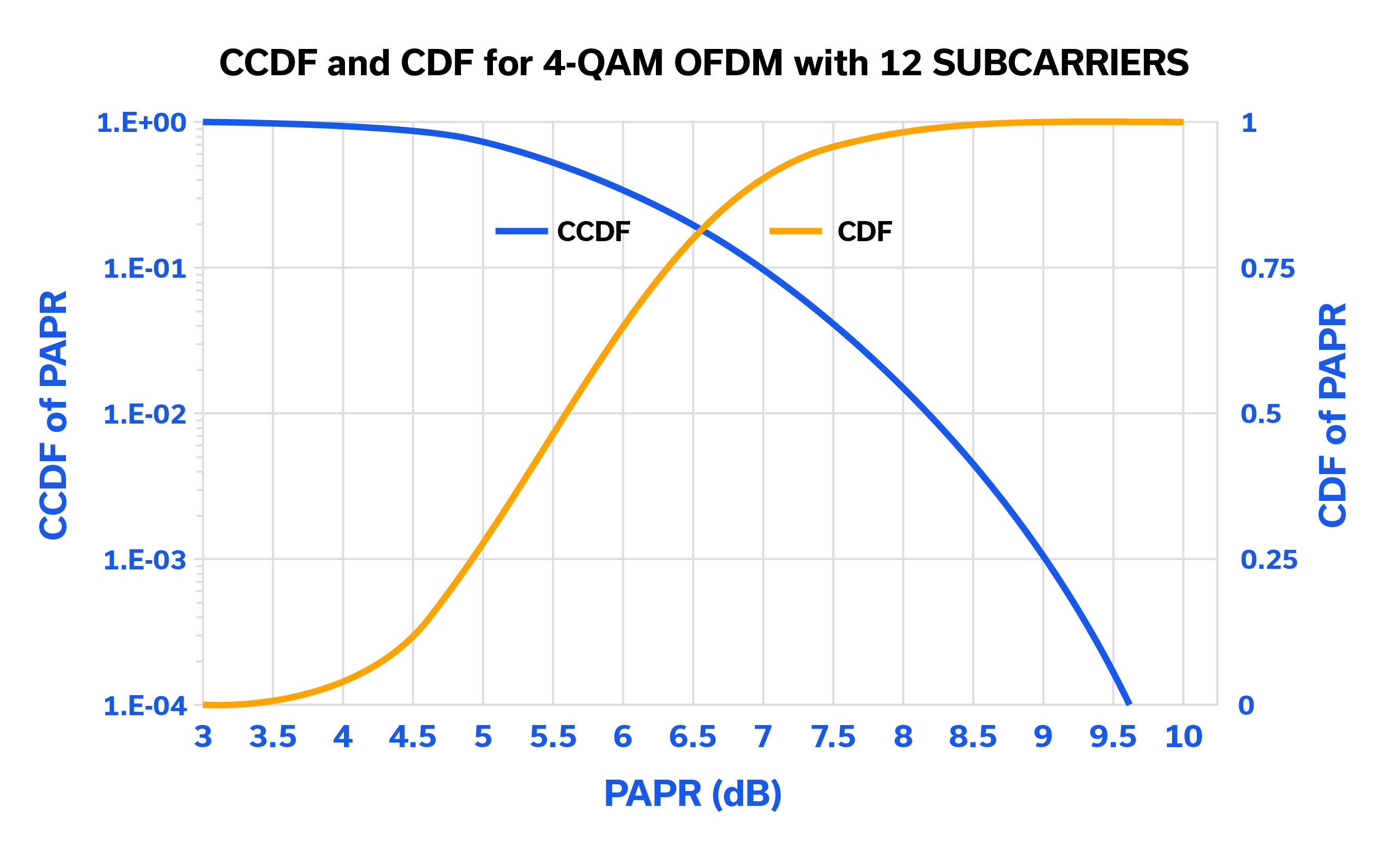
Figure 3: CCDF (log scale) and CDF (linear scale) for 4-QAM OFDM waveform with 12 subcarriers

The Complementary Cumulative Distribution Function (CCDF)

In most cases, such as designing an RF amplifier, it is more useful to know how often the RF signal power will be above a certain value. The complementary cumulative distribution function (CCDF) is obtained by calculating: CCDF = (1 – CDF). Using the previous example of a power level of 0 dBm, referencing the CCDF curve yields the probability of 0.1 that the RF power will be above 0 dBm 10 percent of the time. These two points on their respective curves both occur at a PAPR of approximately 7 dB.

CCDF curves generally show the PAPR of a signal. A signal with constant PAPR over time, such as GSM, will be a near-vertical line on the CCDF graph. As the PAPR increases, the curve shifts right, indicating additional stress on RF system components. Modern RF modulation schemes, such as LTE and 5G, can have PAPRs well over 10 dB.

CCDF, with its graphical representation of PAPR, makes the analysis of RF signals more intuitive. The horizontal axis (power or PAPR) can be expressed in absolute or relative values. If the input signal and output signal of an RF component differ significantly, this may indicate compression. Measuring the input CCDF and output CCDF can show that peak power excursions are being clipped, as the low-probability portion of the PAPR curve goes vertical.

Complimentary Summary

CCDF is a useful graphical tool for assessing and quantifying the performance of RF components. This statistical approach allows a wide range of signal PAPRs to be analyzed rather than a single value. As modern RF signals continue to evolve and measurements become more challenging, CCDF remains an intuitive way to gauge RF system performance.

References

1. OFDM signal in time domain
2. Probability Density Function
3. How to Find Probability Density Function
4. Waveform and Space Precoding for Next Generation Downlink Narrowband IoT, Xu, Masouros, and Darwazeh
5. CDF of PAPR for OFDM and SEFDM

Get in touch for orders or any queries: sales@rfdesign.co.za / +27 21 555 8400

Courtesy of Mini-Circuits